😀 본 예제는 kaggle 의 EDA & ML 코드의 best practice를 보며 스터디한 내용입니다.
- 전체적인 코드는 이 링크로 >> https://www.kaggle.com/code/oscarm524/ps-s3-ep16-eda-modeling-submission/notebook
🦀 이번 시간에는 '게' 나이를 예측하는 것을 주제로 데이터를 탐색하고,
EDA를 하는 기초적인 과정을 살펴본다

라이브러리 load
import pandas as pd
import numpy as np
import matplotlib.pyplot as plt; plt.style.use('ggplot')
import seaborn as sns
import plotly.express as px
from sklearn.tree import DecisionTreeRegressor, plot_tree
from sklearn.model_selection import KFold, StratifiedKFold, train_test_split, GridSearchCV
from sklearn.tree import DecisionTreeRegressor, plot_tree
from sklearn.preprocessing import MinMaxScaler, StandardScaler, LabelEncoder
from sklearn.pipeline import make_pipeline
from sklearn.linear_model import Ridge, RidgeCV, Lasso, LassoCV
from sklearn.model_selection import KFold, StratifiedKFold, train_test_split, GridSearchCV, RepeatedKFold, RepeatedStratifiedKFold
from sklearn.metrics import mean_squared_error, mean_absolute_error
from sklearn.inspection import PartialDependenceDisplay
from sklearn.ensemble import RandomForestRegressor, HistGradientBoostingRegressor, GradientBoostingRegressor, ExtraTreesRegressor
from sklearn.svm import SVR

from lightgbm import LGBMRegressor
from xgboost import XGBRegressor
from catboost import CatBoostRegressor
from sklego.linear_model import LADRegression
Data 불러오고 기초 통계량 확인
- 데이터를 로드한 뒤에는 먼저 전체적인 크기(shape)을 확인한다 : 행과 열 개수
train = pd.read_csv('train.csv')
original = pd.read_csv('CrabAgePrediction.csv')
test = pd.read_csv('test.csv')
submission = pd.read_csv('sample_submission.csv')

print('train data size : ', train.shape)
print('test data size : ', test.shape)
print('submission data size : ', submission.shape)
결과 예시
train data size :  (74051, 10)
test data size :  (49368, 9)
submission data size :  (49368, 2)
- head() 로 첫 5줄의 데이터를 출력해서 확인하고, describe() 로 수치형 값들의 기초 통계량을 확인
- 이때, 결측치의 분포도 함께 확인할 수 있다
train.head()
train.describe()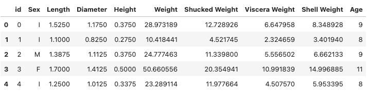
Data 탐색
1. 중복값 확인
- drop.duplicates()를 사용하여, 전체 데이터 사이즈에서 중복값을 빼고 난 후의 사이즈(행의 개수)를 비교한다
- 이를 통해 전체 데이터에서 중복된 값이 있는지 볼 수 있다
print(f'There are {train.shape[0]} observations in the train dataset')
print('There are', train.drop(columns=['id'], axis = 1).drop_duplicates().shape[0], 'unique observations in the train dataset')
print('There are', train.drop(columns=['id', 'Age'], axis = 1).drop_duplicates().shape[0], 'unique observations (only features) in the trian dataset')
2. 데이터의 분포 확인
- 기본적으로 train, test 데이터의 분포와 컬럼간 상관관계를 확인한다
- 특히 대회제출용 데이터는 train, test가 따로 나뉘어 있으니 이를 유의하여 체크한다
- 본 포스팅의 데이터는 train, original, test 이렇게 3개의 데이터 셋을 기본으로 한다.
- train 데이터는 original 데이터에서 추출된 것으로 예상되며, 정확한 분석을 위해 train과 original 데이터의 전체적인 분포나 상태를 확인하는 것이다.
fig, axes = plt.subplots(1, 2, figsize = (18, 8))

sns.kdeplot(ax = axes[0], data = train, x = 'Age', fill = True, color = 'steelblue').set_title('train data');
sns.kdeplot(ax = axes[1], data = original, x = 'Age', fill = True, color = 'orange').set_title('original data');
plt.show()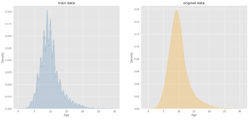
👉 두 데이터의 분포가 전체적으로 동일하다
3. 데이터 컬럼과 target의 상관관계 확인
corr_train = train.drop(columns = ['id', 'Sex'], axis = 1).corr()
corr_original = original.drop(columns = ['Sex'], axis = 1).corr()

train_mask = np.triu(np.ones_like(corr_train, dtype = bool))
original_mask = np.triu(np.ones_like(corr_original, dtype = bool))

cmap = sns.diverging_palette(100, 7, s = 75, l = 40, n = 20, center = 'light', as_cmap = True)

fig, axes = plt.subplots(1, 2, figsize = (25, 10))
sns.heatmap(corr_train, annot = True, cmap = cmap, fmt = '.2f', center = 0,
            annot_kws = {'size':12}, ax = axes[0], mask = train_mask).set_title('train 상관관계')

sns.heatmap(corr_original, annot = True, cmap = cmap, fmt = '.2f', center = 0,
           annot_kws = {'size':12}, ax = axes[1], mask = original_mask).set_title('original 상관관계')

plt.show()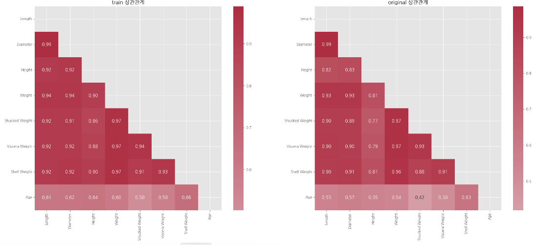
👉 두 데이터의 상관계수도 유사하게 나타난다
- age와 shell weight의 상관계수가 가장 높음
- age 와 shucked weight의 상관계수가 가장 낮음
4. 주요 컬럼과 target의 관계 시각화
4-1. Sex - Age
# sex컬럼을 범주형 데이터로 변환, I/M/F 순서의 범주를 가지도록 함(시각화용)
original['Sex'] = pd.Categorical(original['Sex'], categories = ['I', 'M', 'F'], ordered = True)

fig, axes = plt.subplots(1, 2, figsize = (15, 6))

sns.boxplot(ax = axes[0], data = train, x = 'Sex', y = 'Age').set_title('Competition Dataset')
sns.boxplot(ax = axes[1], data = original, x = 'Sex', y = 'Age').set_title('Original Dataset');
👉 성별이 명확히 구분된 경우, 유사한 분포를 보임
4-2. Shell Weight - Age
fig, axes = plt.subplots(1, 2, figsize = (15, 6))

sns.scatterplot(ax = axes[0], data = train, x = 'Shell Weight', y = 'Age', color = 'steelblue').set_title('Competition Dataset')
sns.scatterplot(ax = axes[1], data = original, x = 'Shell Weight', y = 'Age', color = 'orange').set_title('Original Dataset');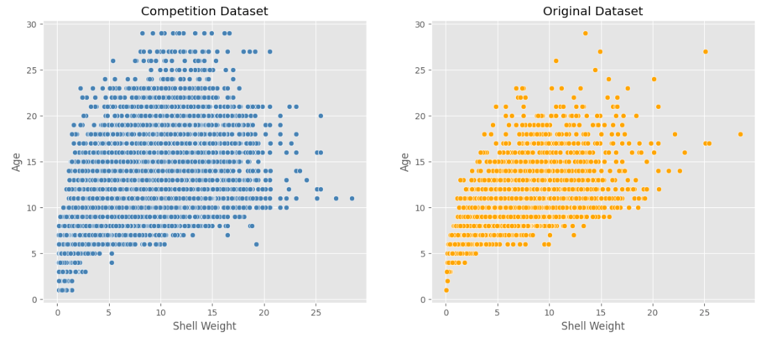
👉 양의 상관관계
4-3. Diameter - Age
fig, axes = plt.subplots(1, 2, figsize = (15, 6))

sns.scatterplot(ax = axes[0], data = train, x = 'Diameter', y = 'Age', color = 'steelblue').set_title('Competition Dataset')
sns.scatterplot(ax = axes[1], data = original, x = 'Diameter', y = 'Age', color = 'orange').set_title('Original Dataset');
👉 양의 상관관계(선형)
다음 포스팅에서는 이를 바탕으로 다양한 모델을 기반으로한 baseline code를 짜보는 것으로 이어진다!
728x90
'Machine Learning > Case Study 👩🏻💻' 카테고리의 다른 글
| [🦀 게 나이 예측(3)] Baseline Modeling(Hist Gradient Boosting) (2) | 2023.09.24 |
|---|---|
| [🦀 게 나이 예측(2)] Baseline Modeling(Gradient Boosting) (0) | 2023.09.24 |
| [중고차 가격 예측(2)] EDA (0) | 2023.09.17 |
| [중고차 가격 예측(1)] pandas_profiling 을 이용한 피쳐 요약 확인 (0) | 2023.09.17 |
| [해외 부동산 월세 예측(2)] One-Hot Encoding & Ridge Regression (0) | 2023.09.15 |


