
Data Load
- 8692개의 데이터
- ID : 샘플 별 고유 ID
- 부동산 관련 정보
- 해당 건물이 위치한 위도와 경도(단, 지도 api를 이용하여 추가정보를 활용할 수 없음)
- target: monthlyRent(us_dollar) : 1달러를 단위로 하는 월세 가격

기본적인 EDA
▶︎ 질적 변수와 양적 변수 확인
# 질적 변수
qual_df = total_df[['propertyType', 'suburbName']]

# 양적 변수
quan_df = total_df.drop(columns = ['propertyType', 'suburbName'])
▶︎ 결측치, 행과 컬럼 구성, 데이터타입 / 통계량 확인

▶︎ 시각화
1) 양적 변수 분포 확인 : 히스토그램
quan_df.hist(bins = 100, figsize = (18, 18))
plt.show()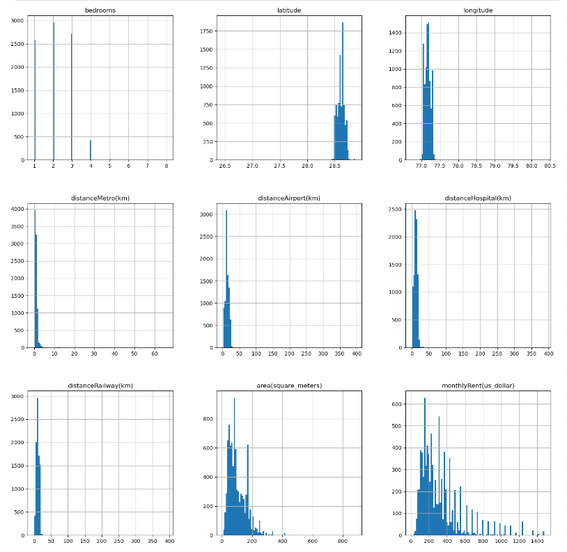
2) 질적 변수 분포 확인 : countplot
- 질적 변수는 수치화가 되지 않으면 히스토그램으로 나타낼 수 없다
- 그러나 단순 수치화가 질적 변수의 특성을 적절하게 반영하지 못할 때가 많으므로,
- 질적변수는 관측값의 빈도를 나타내는 countplot을 주로 이용한다
fig, axes = plt.subplots(2, 1, figsize = (20, 15))

sns.countplot(x = qual_df['propertyType'],ax = axes[0])
sns.countplot(x = qual_df['suburbName'], ax = axes[1])

plt.show()
3) 이상치 확인 : box plot
# 일부 코드
fig, axes = plt.subplots(3, 3, figsize = (15, 15))

sns.boxplot(y = quan_df['bedrooms'], ax = axes[0][0])
sns.boxplot(y = quan_df['latitude'], ax=axes[0][1])
sns.boxplot(y = quan_df['longitude'], ax=axes[0][2])
plt.show()
4) 상관관계 확인 : heatmap
plt.figure(figsize = (15, 15))
sns.heatmap(total_df.corr(), annot = True, fmt = '.1f', linewidth = 1, cmap = 'Blues')
plt.show()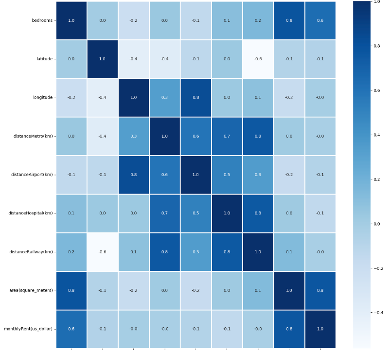
728x90
'Machine Learning > Case Study 👩🏻💻' 카테고리의 다른 글
| [🦀 게 나이 예측(2)] Baseline Modeling(Gradient Boosting) (0) | 2023.09.24 |
|---|---|
| [🦀 게 나이 예측(1)] 데이터 탐색 & EDA (0) | 2023.09.24 |
| [중고차 가격 예측(2)] EDA (0) | 2023.09.17 |
| [중고차 가격 예측(1)] pandas_profiling 을 이용한 피쳐 요약 확인 (0) | 2023.09.17 |
| [해외 부동산 월세 예측(2)] One-Hot Encoding & Ridge Regression (0) | 2023.09.15 |


